Scikit-learn is a powerful machine learning library that provides a wide variety of modules for data access, data preparation and statistical model building. It has a good selection of clean toy data sets that are great for people just getting started with data analysis and machine learning. Even better, easy access to these data sets removes the hassle of searching for and downloading files from an external data source. The library also enables data processing tasks such as imputation, data standardization and data normalization. These tasks can often lead to significant improvements in model performance.
Scikit-learn also provides a variety of packages for building linear models, tree-based models, clustering models and much more. It features an easy-to-use interface for each model object type, which facilitates fast prototyping and experimentation with models. Beginners in machine learning will also find the library useful since each model object is equipped with default parameters that provide baseline performance. Overall, Scikit-learn provides many easy-to-use modules and methods for accessing and processing data and building machine learning models in Python. This tutorial will serve as an introduction to some of its functions.
Scikit-Learn Overview
Scikit-learn Data Sets
Scikit-learn provides a wide variety of toy data sets, which are simple, clean, sometimes fictitious data sets that can be used for exploratory data analysis and building simple prediction models. The ones available in Scikit-learn can be applied to supervised learning tasks such as regression and classification.
For example, it has a set called iris data, which contains information corresponding to different types of iris plants. Users can employ this data for building, training and testing classification models that can classify types of iris plants based on their characteristics.
Scikit-learn also has a Boston housing data set, which contains information on housing prices in Boston. This data is useful for regression tasks like predicting the dollar value of a house. Finally, the handwritten digits data set is an image data set that is great for building image classification models. All of these data sets are easy to load using a few simple lines of Python code.
To start, let’s walk through loading the iris data. We first need to import the pandas and numpy packages:
import pandas as pd

import numpy as np
Next, we relax the display limits on the columns and rows:
pd.set_option('display.max_columns', None)

pd.set_option('display.max_rows', None)
We then load the iris data from Scikit-learn and store it in a pandas data frame:
from sklearn.datasets import load_iris

data = load_iris()

df = pd.DataFrame(data.data,columns=data.feature_names)

df['target'] = pd.Series(data.target)
Finally, we print the first five rows of data using the head() method:
print(df.head())
We can repeat this process for the Boston housing data set. To do so, let’s wrap our existing code in a function that takes a Scikit-learn data set as input:
def get_data(dataset):

    data = dataset

    df = pd.DataFrame(data.data,columns=data.feature_names)

    df['target'] = pd.Series(data.target)

    print(df.head())
We can call this function with the iris data and get the same output as before:
get_data(load_iris())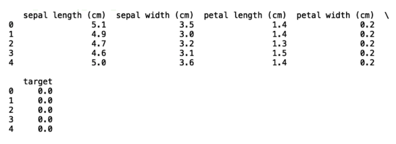
Now that we see that our function works, let’s import the Boston housing data and call our function with the data:
from sklearn.datasets import load_iris, load_boston

get_data(load_boston())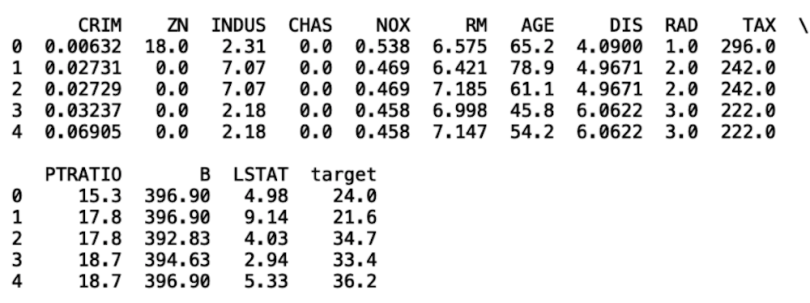
Finally, let’s load the handwritten digits data set, which contains images of handwritten digits from zero through nine. Since this is an image data set, it’s neither necessary nor useful to store it in a data frame. Instead, we can display the first five digits in the data using the visualization library matplotlib:
from sklearn.datasets import load_iris, load_boston, load_digits

import matplotlib.pyplot as plt

def get_data(dataset):

    try:

        data = dataset

        df = pd.DataFrame(data.data,columns=data.feature_names)

        df['target'] = pd.Series(data.target)

        print(df.head())

    except(AttributeError):

        data = dataset

        plt.gray()

        for i in range(0,5):

            plt.matshow(data.images[i])

            plt.show()
And if we call our function with load_digits(), we get the following displayed images:

I can’t overstate the ease with which a beginner in the field can access these toy data sets. These sets allow beginners to quickly get their feet wet with different types of data and use cases such as regression, classification and image recognition.
Data Imputation
Scikit-learn also provides a variety of methods for data processing tasks. First, let’s take a look at data imputation, which is the process of replacing missing data and is important because oftentimes real data contains either inaccurate or missing elements. This can result in misleading results and poor model performance.
Being able to accurately impute missing values is a skill that both data scientists and industry domain experts should have in their toolbox. To demonstrate how to perform data imputation using Scikit-learn, we’ll work with the University of California–Irvine’s data set on housing electric power consumption, which is available here. Since the data set is quite large, we’ll take a random sample of 40,000 records for simplicity and store the down-sampled data in a separate csv file called “hpc.csv”:
df = pd.read_csv('household_power_consumption.txt', sep=';')

df = df.sample(40000)

df.to_csv('hpc.csv')

Next, let’s read in our newly created data set and print the first five rows:

df = pd.read_csv('hpc.csv')

print(df.head())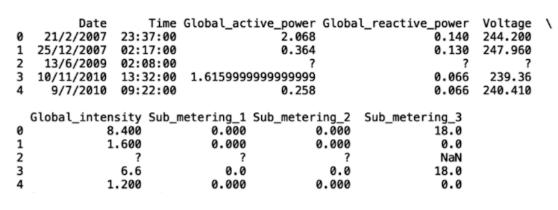
As we can see, the third row (second index) contains missing values specified by ? and NaN. The first thing we can do is replace the ? values with NaN values. Let’s demonstrate this with Global_active_power:
df['Global_active_power'].replace('?', np.nan, inplace = True)

print(df.head())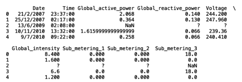
We can repeat this process for the rest of the columns:
df['Global_reactive_power'].replace('?', np.nan, inplace = True)

df['Voltage'].replace('?', np.nan, inplace = True)

df['Global_intensity'].replace('?', np.nan, inplace = True)

df['Sub_metering_1'].replace('?', np.nan, inplace = True)

df['Sub_metering_2'].replace('?', np.nan, inplace = True)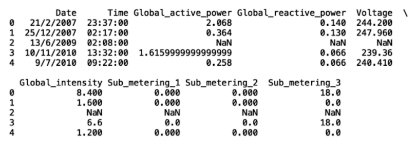
Now, to impute the missing values, we import the SimpleImputer method from Scikit-learn. We will define an imputer object that simply imputes the mean for missing values:
from sklearn.impute import SimpleImputer

imp_mean = SimpleImputer(missing_values=np.nan, strategy='mean')
And we can fit our imputer to our columns with missing values:
X = df[['Global_active_power', 'Global_reactive_power', 'Voltage', 'Global_intensity', 'Sub_metering_1','Sub_metering_2' ]]

imp_mean.fit(X)
Store the result in a data frame:
df_new = pd.DataFrame(imp_mean.transform(X), columns = ['Global_active_power', 'Global_reactive_power', 'Voltage',

                      'Global_intensity', 'Sub_metering_1','Sub_metering_2' ])
Add back the additional date and time columns:
df_new['Date'] = df['Date']

df_new['Time'] = df['Time']
And print the first five rows of our new data frame:
print(df_new.head())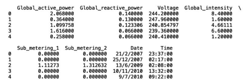
As we can see, the missing values have been replaced.
Although Scikit-learn’s SimpleImputer isn’t the most sophisticated imputation method, it removes much of the hassle around building a custom imputer. This simplicity is useful for beginners who are dealing with missing data for the first time. Further, it serves as a good demonstration of how imputation works. By introducing the process, it can motivate more sophisticated extensions of this type of imputation such as using a statistical model to replace missing values.
Data Standardization and Normalization
Data standardization and normalization are also easy with Scikit-learn. Both of these are useful in machine learning methods that involve calculating a distance metric like K-nearest neighbors and support vector machines. They’re also useful in cases where we can assume the data is normally distributed and for interpreting coefficients in linear models to be of variable importance.
Standardization
Standardization is the process of subtracting values in numerical columns by the mean and scaling to unit variance (through dividing by the standard deviation). Standardization is necessary in cases where a wide range of numerical values may artificially dominate prediction outcomes.
Let’s consider standardizing the Global_intensity in the power consumption data set. This column has values ranging from 0.2 to 36. First, let’s import the StandardScalar() method from Scikit-learn:
scaler = StandardScaler()

scaler.fit(np.array(df_new[['Global_intensity']]))

df_new['Global_intensity'] = scaler.transform(np.array(df_new[['Global_intensity']]))

Now we see that the min and max are 7.6 and -1.0:

print(df_new.head())

print("Max: ", df_new['Global_intensity'].max())

print("Min: ", df_new['Global_intensity'].min())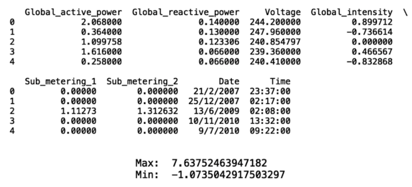
Normalization
Data normalization scales a numerical column such that its values are between 0 and 1. Normalizing data using Scikit-learn follows similar logic to standardization. Let’s apply the normalizer method to the Sub_metering_2 column:
from sklearn.preprocessing import Normalizer

normalizer = Normalizer()

normalizer.fit(np.array(df_new[['Sub_metering_2']]))

df_new['Sub_metering_2'] = normalizer.transform(np.array(df_new[['Sub_metering_2']]))

print(df_new.head())

print("Max: ", df_new['Sub_metering_2'].max())

print("Min: ", df_new['Sub_metering_2'].min())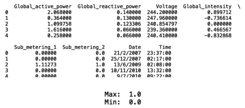
Now we see that the min and max are 1.0 and 0.
In general, you should standardize data if you can safely assume it’s normally distributed. Conversely, if you can safely assume that your data isn’t normally distributed, then normalization is a good method for scaling it. Given that these transformations can be applied to numerical data with just a few lines of code, the StandardScaler() and Normalizer() methods are great options for beginners dealing with data fields that have widely varying values or data that isn’t normally distributed.
Statistical Modeling With Scikit-Learn
Scikit-learn also has methods for building a wide array of statistical models, including linear regression, logistic regression and random forests. Linear regression is used for regression tasks. Specifically, it works for the prediction of continuous output like housing price, for example. Logistic regression is used for classification tasks in which the model predicts binary output or multiclass like predicting iris plant type based on characteristics. Random forests can be used for both regression and classification. We’ll walk through how to implement each of these models using the Scikit-learn machine learning library in Python.
Linear Regression
Linear regression is a statistical modeling approach in which a linear function represents the relationship between input variables and a scalar response variable. To demonstrate its implementation in Python, let’s consider the Boston housing data set. We can build a linear regression model that uses age as an input for predicting the housing value. To start, let’s define our input and output variables:
X = df_housing[['AGE']]

y = df_housing[['target']]
Next, let’s split our data for training and testing:
from sklearn.model_selection import train_test_split

X_train, y_train, X_test, y_test = train_test_split(X, y, random_state = 42)
Now let’s import the linear regression module from Scikit-learn:
from sklearn.linear_models import LinearRegressionFinally, let’s train, test and evaluate the performance of our model using R^2 and RMSE:
linear_model = LinearRegression()

linear_model.fit(X_train, y_train)

y_pred = linear_model.predict(X_test)

from sklearn.metrics import mean_squared_error

from sklearn.metrics import r2_score

rms = mean_squared_error(y_test, y_pred)

r2 =  r2_score(y_test, y_pred)

print("MSE:", rms)

print("R^2:", r2)
Since we use one variable to predict a response, this is a simple linear regression. But we can also use more than one variable in a multiple linear regression. Let’s build a linear regression model with age (AGE), average number of rooms (RM), and pupil-to-teacher ratio (PTRATION). All we need to do is redefine X (input) as follows:
X = df_housing[['AGE', 'PTRATIO', 'RM']]This gives the following improvement in performance:

Linear regression is a great method to use if you’re confident that there is a linear relationship between input and output. It’s also useful as a benchmark against more sophisticated methods like random forests and support vector machines.
Logistic Regression
Logistic regression is a simple classification model that predicts binary or even multiclass output. The logic for training and testing is similar to linear regression.
Let’s consider the iris data for our Python implementation of a logistic regression model. We’ll use sepal length (cm), sepal width (cm), petal length (cm) and petal width (cm) to predict the type of iris plant:
df_iris= get_data(load_iris())

X = df_iris[['sepal length (cm)', 'sepal width (cm) ', 'petal length (cm)', 'petal width (cm)']]

y = df_iris[['target']]

X_train, X_test, y_train, y_test = train_test_split(X, y, random_state = 42)

logistic_model = LogisticRegression()

logistic_model.fit(X_train, y_train)

y_pred = linear_model.predict(X_test)
We can evaluate and visualize the model performance using a confusion matrix:
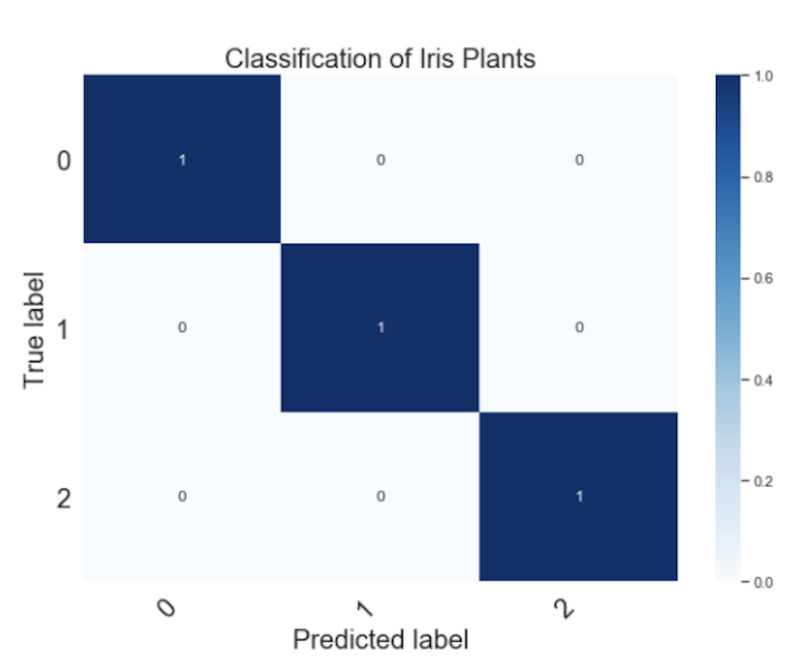
We see that the model correctly captures all of the true positives across the three iris plant classes. Similar to linear regression, logistic regression depends on a linear sum of inputs used to predict each class. As such, logistic regression models are referred to as generalized linear models. Given that logistic regression models a linear relationship between input and output, they’re best employed when you know that there is a linear relationship between input and class membership.
Random Forests
Random forests, also called random decision trees, is a statistical model for both classification and regression tasks. Random forests are basically a set of questions and answers about the data organized in a tree-like structure.
These questions split the data into subgroups so that the data in each successive subgroup are most similar to each other. For example, say we’d like to predict whether or not a borrower will default on a loan. A question that we can ask using historical lending data is whether or not the customer’s credit score is below 700. The data that falls into the “yes” bucket will have more customers who default than the data that falls into the “no” bucket.
Within the yes bucket, we can further ask if the borrower’s income is below $30,000. Presumably, the yes bucket here will have an even greater percentage of customers who default. Decision trees continue asking statistical questions about the data until achieving maximal separation between the data corresponding to those who default and those who don’t.
Random forests extend decision trees by constructing a multitude of them. In each of these trees, we ask statistical questions on random chunks and different features of the data. For example, one tree may ask about age and credit score on a fraction of the train data. Another may ask about income and gender on a separate fraction of the training data, and so forth. Random forest then performs consensus voting across these decision trees and uses the majority vote for the final prediction.
Implementing a random forests model for both regression and classification is straightforward and very similar to the steps we went through for linear regression and logistic regression. Let’s consider the regression task of predicting housing prices using the Boston housing data. All we need to do is import the random forest regressor module, initiate the regressor object, fit, test and evaluate our model:
from sklearn.ensemble import RandomForestRegressor

rf_reg = RandomForestRegressor()

rf_reg.fit(X_train, y_train)

y_pred = rf_reg.predict(X_test)

from sklearn.metrics import mean_squared_error

from sklearn.metrics import r2_score

rms = mean_squared_error(y_test, y_pred)

r2 =  r2_score(y_test, y_pred)

print("RF MSE:", rms)

print("RF R^2:", r2)
We see a slight improvement in performance compared to linear regression.
The random forest object takes several parameters that can be modified to improve performance. The three I’ll point out here are n_estimators, max_depth and random_state. You can check out the documentation for a full description of all random forest parameters.
The parameter n_estimators is simply the number of decision trees that the random forest is made up of. Max_depth measures the longest path from the first question to a question at the base of the tree. Random_state is how the algorithm randomly chooses chunks of the data for question-asking.
Since we didn’t specify any values for these parameters, the random forest module automatically selects a default value for each parameter. The default value for n_estimators is 10, which corresponds to 10 decision trees. The default value for max_depth is None, which means there is no cut-off for the length of the path from the first question to the last question at the base of the decision tree. This can be roughly understood as the limit on the number of questions we ask about the data. The default value for random_state is None. This means, upon each model run, different chunks of data will be randomly selected and used to construct the decision trees in the random forests. This will result in slight variations in output and performance.
Despite using default values, we achieve pretty good performance. This accuracy demonstrates the power of random forests and the ease with which the data science beginner can implement an accurate random forest model.
Let’s see how to specify n_estimators, max_depth and random_state. We’ll choose 100 estimators, a max depth of 10 and a random state of 42:
rf_reg = RandomForestRegressor(n_estimators= 100, max_depth=10, random_state =42)
We see that we get a slight improvement in both MSE and R^2. Further, specifying random_state makes our results reproducible since it ensures the same random chunks of data are used to construct the decision trees.
Applying random forest models to classification tasks is very straightforward. Let’s do this for the iris classification task:
rf_cass = RandomForestClassifier(n_estimators= 100, max_depth=10, random_state =42)

rf_cass.fit(X_train, y_train)

y_pred = rf_cass.predict(X_test)
And the corresponding confusion matrix is just as accurate:
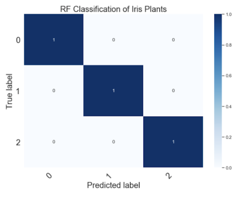
Random forests are a great choice for building a statistical model since they can be applied to a wide range of prediction use cases. This includes classification, regression and even unsupervised clustering tasks. It’s a fantastic tool that every data scientist should have in their back pocket. In the context of Scikit-learn, they’re extremely easy to implement and modify for improvements in performance. This enables fast prototyping and experimentation of models, which leads to accurate results faster.
Finally, all the code in this post is available on GitHub.
Experiment With Scikit-Learn
Overall, Scikit-learn provides many easy-to-use tools for accessing benchmark data, performing data processing, and training, testing and evaluating machine learning models. All of these tasks require relatively few lines of code, making the barrier to entry for beginners in data science and machine learning research quite low. Users can quickly access toy data sets and familiarize themselves with different machine learning use cases (classification, regression, clustering) without the hassle of finding a data source, downloading and then cleaning the data. Upon becoming familiar with different use cases, the user can then easily port over what they’ve learned to more real-life applications.
Further, new data scientists unfamiliar with data imputation can quickly pick up how to use the SimpleImputer package in Scikit-learn and implement some standard methods for replacing missing or bad values in data. This can serve as the foundation for learning more advanced methods of data imputation, such as using a statistical model for predicting missing values. Additionally, the standard scaler and normalizer methods make data preparation for advanced models like neural networks and support vector machines very straightforward. This is often necessary in order to achieve satisfactory performance with more complicated models like support vector machines and neural networks.
Finally, Scikit-learn makes building a wide variety of machine learning models very easy. Although I’ve only covered three in this post, the logic for building other widely used models such as support vector machines and K-nearest neighbors is very similar. It is also very suitable for beginners who have limited knowledge of how these algorithms work under the hood, given that each model object comes with default parameters that give baseline performance. Whether the task is model benching marking with toy data, preparing/cleaning data, or evaluating model performance Scikit-learn is a fantastic tool for building machine learning models for a wide variety of use cases.


