A goal of supervised learning is to build a machine learning model that performs well on new data. If you have new data, it’s a good idea to see how your model performs on it. The problem is that you may not have new data, but you can simulate this experience with a procedure like train test split.
What Is a Train Test Split?
Train test split is a machine learning model validation process that allows you to simulate how your model would perform with new data.
This tutorial includes:
- What is the train test split procedure?
- How to use train test split to tune models in Python.
- Understanding the bias-variance tradeoff.
If you would like to follow along, the code and images used in this tutorial is available on GitHub. With that, let’s get started.
What Is the Train Test Split Procedure?
Train test split is a model validation procedure that allows you to simulate how a model would perform on new/unseen data by splitting a dataset into a training set and a testing set. The training set is data used to train the model, and the testing set data (which is new to the model) is used to test the model’s performance and accuracy. A train test split can also involve splitting data into a validation set, which is data used to fine-tune hyperparameters and optimize the model during the training process.
Here is how the train test split procedure works:
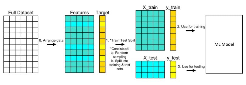
1. Arrange the Data
Make sure your data is arranged into a format acceptable for train test split. In scikit-learn, this consists of separating your full dataset into “Features” and “Target.”
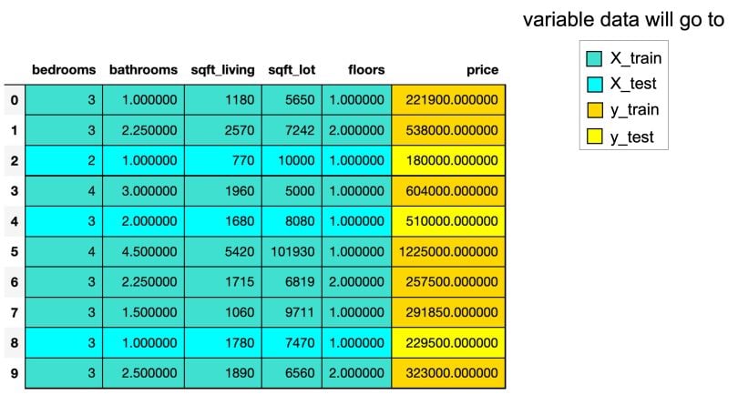
2. Split the Data
Split the dataset into two pieces — a training set and a testing set. This consists of random sampling without replacement about 75 percent of the rows (you can vary this) and putting them into your training set. The remaining 25 percent is put into your test set. Note that the colors in “Features” and “Target” indicate where their data will go (“X_train,” “X_test,” “y_train,” “y_test”) for a particular train test split.
3. Train the Model
Train the model on the training set. This is “X_train” and “y_train” in the image.
4. Test the Model
Test the model on the testing set (“X_test” and “y_test” in the image) and evaluate the performance.
Methods for Splitting Data in a Train Test Split
Different kinds of datasets require different methods for splitting the data into training and testing sets. Here’s some common methods of splitting data in a train test split:
1. Random Splitting
Random splitting involves randomly shuffling data and splitting it into training and testing sets based on given percentages (like 75% training and 25% testing). This is one of the most popular methods for splitting data in train test splits due to it being simple and easy to implement, and is used by default in the scikit-learn train_test_split() method. Random splitting is most effective for large, diverse datasets where categories are generally represented equally in the data.
2. Stratified Splitting
Stratified splitting divides a dataset in a way that preserves its proportion of classes or categories. This creates training and testing sets with class proportions representative of the original dataset. Using stratified splitting can prevent model bias, and is most effective for imbalanced datasets or datasets where categories aren’t represented equally. In a scikit-learn train test split, stratified splitting can be used by specifying the stratify parameter in the train_test_split() method.
3. Time-Based Splitting
Time-based splitting involves organizing data in a set by points in time, ensuring past data is in the training set and future or later data is in the testing set. Splitting data based on time works to simulate real-world scenarios (for example, predicting future financial or market trends) and allows for time series analysis on time series datasets. However, one drawback to time-based splitting is that it may not fully capture trends for non-stationary data (data that continually changes over time). In scikit-learn, time series data can be split into training and testing sets by using the TimeSeriesSplit() method.
Consequences of Not Using Train Test Split
You could try not using train test split and instead train and test the model on the same data. However, I don’t recommend this approach as it doesn’t simulate how a model would perform on new data. It also tends to reward overly complex models that overfit on the dataset, which means a model doesn’t generalize and attempts to fit data too closely to training data.
The steps below go over how this inadvisable process works.
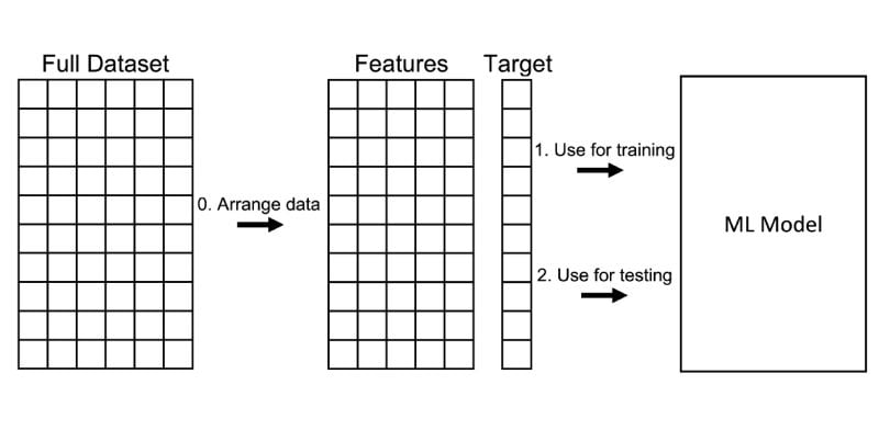
1. Arrange the Data
Make sure your data is arranged into a format acceptable for train test split. In scikit-learn, this consists of separating your full dataset into “Features” and “Target.”
2. Train the Model
Train the model on “Features” and “Target.”
3. Test the Model
Test the model on “Features” and “Target” and evaluate the performance.
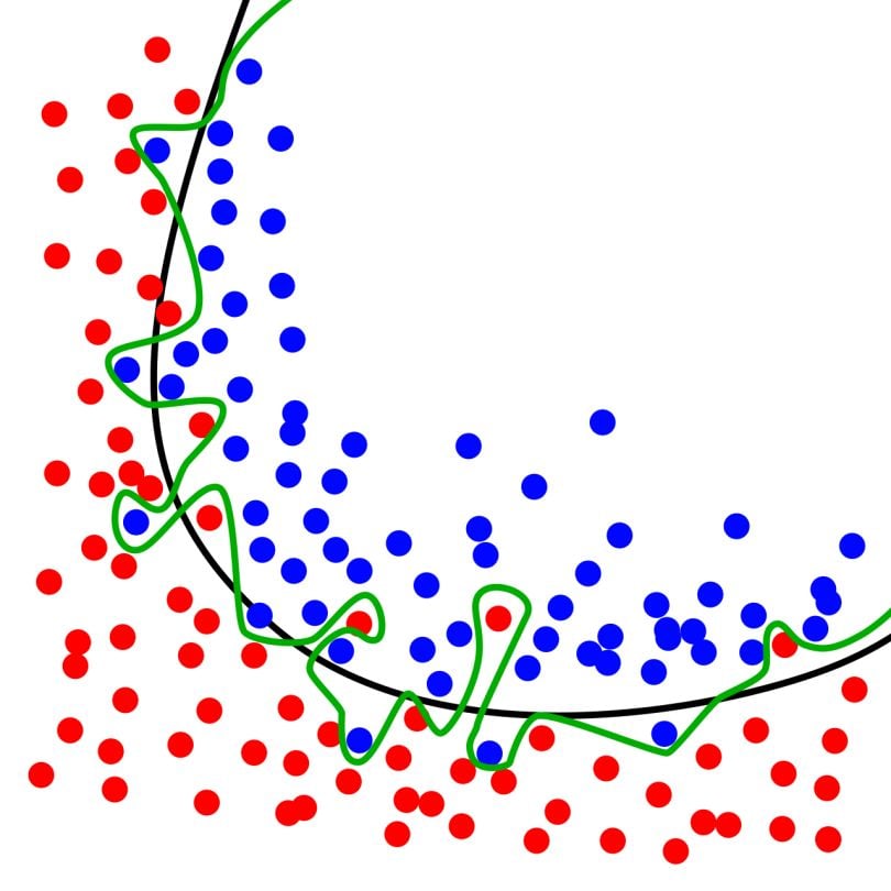
I want to emphasize again that training on an entire dataset and then testing on that same dataset can lead to overfitting. Overfitting is illustrated in the image below. The green squiggly line best follows the training data. The problem is that it is likely overfitting on the training data, meaning it is likely to perform worse on new data.
Using Train Test Split In Python
This section is about the practical application of train test split as a way to predict home prices. It spans everything from importing a dataset to performing a train test split to hyperparameter tuning a decision tree regressor to predicting home prices and more.
Python has a lot of libraries that help you accomplish your data science goals including scikit-learn, pandas, and NumPy, which the code below imports.
import pandas as pd
import numpy as np
import matplotlib.pyplot as plt
from sklearn import tree
from sklearn.model_selection import train_test_split
from sklearn.tree import DecisionTreeRegressor
1. Load the Dataset
Kaggle hosts a dataset which contains the price at which houses were sold for King County, which includes Seattle between May 2014 and May 2015. You can download the dataset from Kaggle or load it from my GitHub. The code below loads the dataset.
url = 'https://raw.githubusercontent.com/mGalarnyk/Tutorial_Data/master/King_County/kingCountyHouseData.csv'
df = pd.read_csv(url)
# Selecting columns I am interested in
columns = ['bedrooms','bathrooms','sqft_living','sqft_lot','floors','price']
df = df.loc[:, columns]
df.head(10)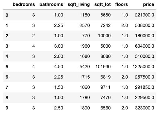
2. Arrange Data into Features and Target
Scikit-learn’s train_test_split() expects data in the form of features and target. In scikit-learn, a features matrix is a two-dimensional grid of data where rows represent samples and columns represent features. A target is what you want to predict from the data. This tutorial uses price as a target.
features = ['bedrooms','bathrooms','sqft_living','sqft_lot','floors']
X = df.loc[:, features]
y = df.loc[:, ['price']]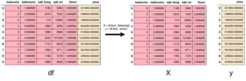
3. Split Data Into Training and Testing Sets
In the code below, train_test_split() splits the data and returns a list which contains four NumPy arrays, while train_size = .75 puts 75 percent of the data into a training set and the remaining 25 percent into a testing set.
X_train, X_test, y_train, y_test = train_test_split(X, y, random_state=0, train_size = .75)The image below shows the number of rows and columns the variables contain using the shape attribute before and after thetrain_test_split.

Shape before and after train_test_split. 75 percent of the rows went to the training set 16209/ 21613 = .75 and 25 percent went to the test set 5404 / 21613 = .25.
4. What Is ‘random_state’ in Train Test Split?
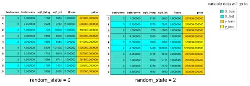
The image above shows that if you select a different value for random_state, different information would go to “X_train,” “X_test,” “y_train” and “y_test”. The random_state is a pseudo-random number parameter that allows you to reproduce the same train test split each time you run the code.
There are a number of reasons why people use random_state, including software testing, tutorials like this one and talks. However, it is recommended you remove it if you are trying to see how well a model generalizes to new data.
Train Test Split: Creating and Training a Model in Scikit-Learn
Here’s what you need to know about using train test split in scikit-learn:
1. Import the Model You Want to Use
In scikit-learn, all machine learning models are implemented as Python classes.
from sklearn.tree import DecisionTreeRegressor2. Make An Instance of the Model
In the code below, I set the hyperparameter max_depth = 2 to pre-prune my tree to make sure it doesn’t have a depth greater than two. The next section of the tutorial will go over how to choose an optimal max_depth for your tree. Also note that I made random_state = 0 so that you can get the same results as me.
reg = DecisionTreeRegressor(max_depth = 2, random_state = 0)3. Train the Model on the Data
Train the model on the data, storing the information learned from the data.
reg.fit(X_train, y_train)4. Predict Labels of Unseen Test Data
# Predicting multiple observations
reg.predict(X_test[0:10])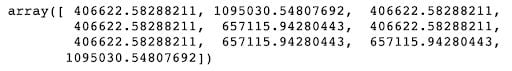
For the multiple predictions above, notice how many times some of the predictions are repeated. If you are wondering why, I encourage you to check out the code below, which will start by looking at a single observation/house and then proceed to examine how the model makes its prediction.
X_test.head(1)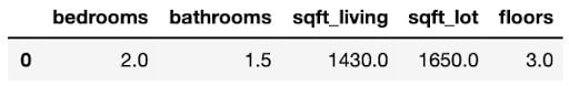
The code below shows how to make a prediction for that single observation.
# predict 1 observation.
reg.predict(X_test.iloc[0].values.reshape(1,-1))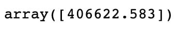
The image below shows how the trained model makes a prediction for the one observation.
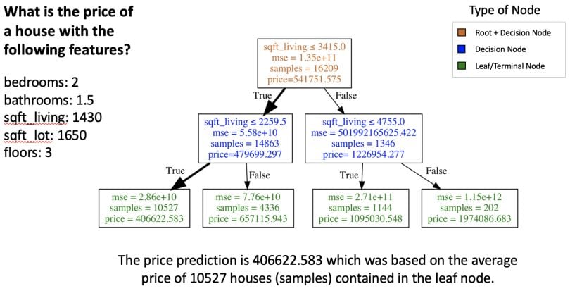
If you are curious how these sorts of diagrams are made, consider checking out my tutorial Visualizing Decision Trees using Graphviz and Matplotlib.
Measuring Train Test Split Model Performance
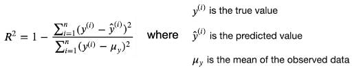
While there are other ways of measuring model performance such as root-mean-square error, and mean absolute error, we are going to keep this simple and use R² — known as the coefficient of determination — as our metric.
The best possible score is 1.0. A constant model that would always predict the mean value of price would get a R² score of 0.0. However, it is possible to get a negative R² on the test set. The code below uses the trained model’s score method to return the R² of the model that we evaluated on the test set.
score = reg.score(X_test, y_test)
print(score)![]()
You might be wondering if our R² above is good for our model. In general, the higher the R², the better the model fits the data. Determining whether a model is performing well can also depend on your field of study. Something harder to predict will generally have a lower R². My argument is that for housing data, we should have a higher R² based solely on our data.
Domain experts generally agree that one of the most important factors in housing prices is location. After all, if you are looking for a home, you’ll most likely care where it’s located. As you can see in the trained model below, the decision tree only incorporates sqft_living.
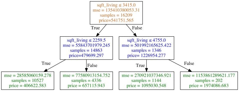
Even if the model was performing very well, it is unlikely that it would get buy-in from stakeholders or coworkers since there is more to a home than sqft_living.
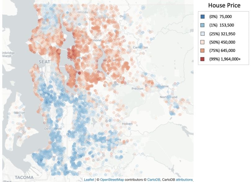
Note that the original dataset has location information like “lat” and “long.” The image below visualizes the price percentile of all the houses in the dataset based on “lat” and “long,” neither were included in the data the model trained on. As you can see, there is a relationship between home price and location.
You can incorporate location information like “lat” and “long” as a way to improve the model. It’s likely places like Zillow found a way to incorporate that into their models.
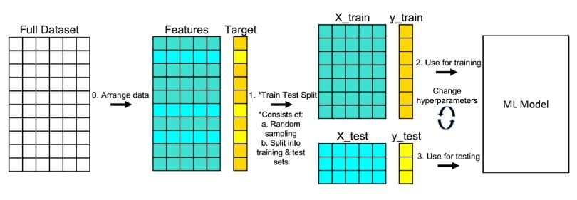
How to Tune the ‘max_depth’ of a Tree
The R² for the model trained earlier in the tutorial was about .438. However, suppose we want to improve the performance so that we can better make predictions on unseen data. While we could add more features like “lat” and “long” to the model or increase the number of rows in the dataset (i.e. find more houses), we could also improve performance through hyperparameter tuning.
This involves selecting the optimal values of tuning parameters for a machine learning problem, which are often called hyperparameters. But first, we need to briefly go over the difference between parameters and hyperparameters. Parameters vs. Hyperparameters
A machine learning algorithm estimates model parameters for a given dataset and updates these values as it continues to learn. You can think of a model parameter as a learned value from applying the fitting process. For example, in logistic regression you have model coefficients. In a neural network, you can think of neural network weights as a parameter. Hyperparameters or tuning parameters are metaparameters that influence the fitting process itself.
For logistic regression, there are many hyperparameters like regularization strength C. For a neural network, there are many hyperparameters like the number of hidden layers. If all of this sounds confusing, Jason Brownlee, founder of Machine Learning Mastery, offers a good rule of thumb in his guide on parameters and hyperparameters which is: “If you have to specify a model parameter manually, then it is probably a model hyperparameter.”
Hyperparameter Tuning
There are a lot of diff erent ways to hyperparameter tune a decision tree for regression. One way is to tune the max_depth hyperparameter. The max_depth (hyperparameter) is not the same thing as depth (parameter of a decision tree), but max_depth is a way to pre-prune a decision tree. In other words, if a tree is already as pure as possible at a depth, it will not continue to split. If this isn’t clear, check out my Understanding Decision Trees for Classification (Python) tutorial to see the difference between max_depth and depth.
The code below outputs the accuracy for decision trees with different values for max_depth.
max_depth_range = list(range(1, 25))
# List to store the average RMSE for each value of max_depth:
r2_list = []
for depth in max_depth_range:
    reg = DecisionTreeRegressor(max_depth = depth,
                            random_state = 0)
    reg.fit(X_train, y_train)

    score = reg.score(X_test, y_test)
    r2_list.append(score)
The graph below shows that the best model R² is when the hyperparameter max_depth is equal to 5. This process of selecting the best model max_depth (max_depth = 5 in this case) among many other candidate models (with different max_depth values in this case) is called model selection.
fig, ax = plt.subplots(nrows = 1, ncols = 1,
                       figsize = (10,7),
                       facecolor = 'white');
ax.plot(max_depth_range,
       r2_list,
       lw=2,
       color='r')
ax.set_xlim([1, max(max_depth_range)])
ax.grid(True,
       axis = 'both',
       zorder = 0,
       linestyle = ':',
       color = 'k')
ax.tick_params(labelsize = 18)
ax.set_xlabel('max_depth', fontsize = 24)
ax.set_ylabel('R^2', fontsize = 24)
ax.set_title('Model Performance on Test Set', fontsize = 24)
fig.tight_layout()
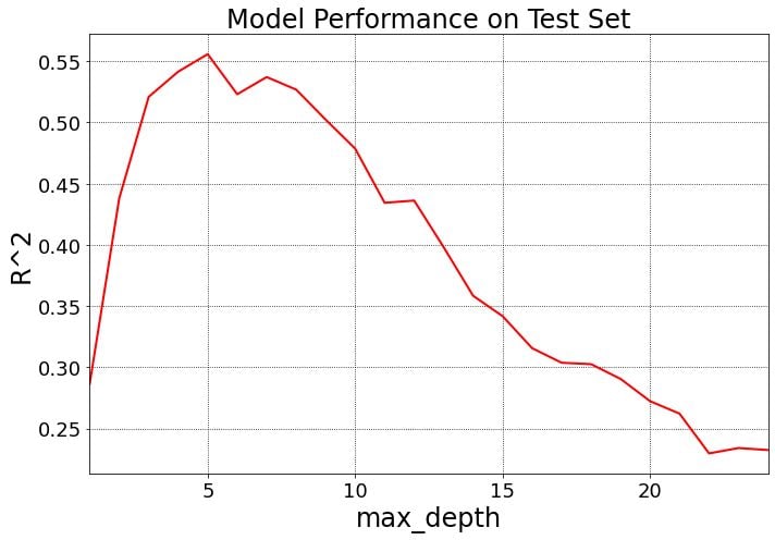
Note that the model above could have still been overfitted on the test set since the code changed max_depth repeatedly to achieve the best model. In other words, knowledge of the test set could have leaked into the model as the code iterated through 24 different values for max_depth (the length of max_depth_range is 24). This would lessen the power of our evaluation metric R², as it would no longer be as strong an indicator of generalization performance. This is why in real life, we often have training, test and validation sets when hyperparameter tuning.
Understanding the Bias-Variance Tradeoff
In order to understand why max_depth of 5 was the “Best Model” for our data, take a look at the graph below, which shows the model performance when tested on the training and test set.
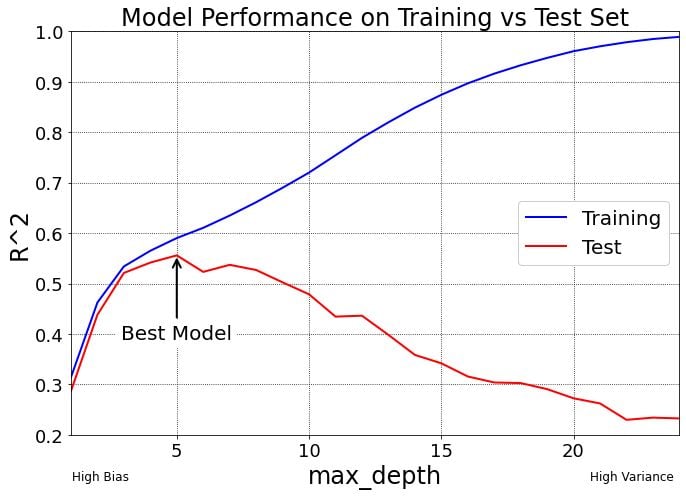
Naturally, the training R² is always better than the test R² for every point on this graph because the models are making predictions on data they have seen before.
To the left side of the “Best Model” on the graph (anything less than max_depth = 5), we have models that underfit the data and are considered high bias because they do not have enough complexity to learn enough about the data.
To the right side of the “Best Model” on the graph (anything more than max_depth = 5), we have models that overfit the data and are considered high variance because they are overly-complex models. These models perform well on the training data but badly on testing data.
The “Best Model” is formed by minimizing bias error — or bad assumptions in the model — and variance error — or oversensitivity to small fluctuations/noise in the training set.
Train Test Split Advantages and Disadvantages
A goal of supervised learning is to build a model that performs well on new data, which train test split helps you simulate. With any model validation procedure it’s important to keep in mind the advantages and disadvantages.
Advantages of a Train Test Split
The advantages of using a train test split include:
- Improved model accuracy and efficiency.
- Reduced model overfitting.
- A relatively fast way to evaluate model performance with new data.
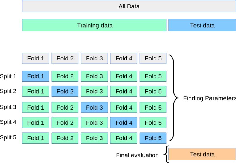
- Simplicity and ease of understanding compared to other methods, such as K-fold cross validation.
- Avoidance of overly complex models that don’t generalize well to new data.
Disadvantages of a Train Test Split
The disadvantages of using a train test split include:
- High variance, as results may vary depending on the specific train test split (
random_state). - Unreliable model performance results when using a dataset that is too small.
- Loss of data that could have been used for training a machine learning model, since testing data isn’t used for training.
- Risk of data leakage during hyperparameter tuning, where knowledge of the test set influences the model. This can be partially solved by using separate training, test, and validation sets.
Frequently Asked Questions
What is a train test split?
A train test split is a machine learning technique used in model validation that simulates how a model would perform with new data. In a train test split, data is split into a training set and a testing set (and sometimes a validation set) using random sample splitting without replacement, stratified splitting or time-based splitting. The model is then trained on the training set, has its performance evaluated using the testing set and is fine-tuned when using a validation set.
What is the default train test split?
The default train test split in scikit-learn splits a dataset into 75% training data and 25% testing data. It is also common to split data into 80% training data and 20% testing data in a train test split. The data split percentages for a train test split can depend on the dataset and model needs.
Is 80% train and 20% test split considered a good practice?
Yes, splitting a dataset in a train test split to be 80% training data and 20% testing data is generally considered a good practice. It’s normally recommended to have a split of 70% to 80% training data and 20% to 30% testing data in a train test split, though these percentages can vary based on dataset size and other model needs.