Understanding the RMSprop Optimizer: A Guide

Root mean square propagation (RMSProp) is an adaptive learning rate optimization algorithm designed to improve training and convergence speed in deep learning models.

If you are familiar with deep learning models, particularly deep neural networks, you know that they rely on optimization algorithms to minimize the loss function and improve model accuracy. Traditional gradient descent methods, such as Stochastic Gradient Descent (SGD), update model parameters by computing gradients of the loss function and adjusting weights accordingly. However, vanilla SGD struggles with challenges like slow convergence, poor handling of noisy gradients, and difficulties in navigating complex loss surfaces.

RMSProp Algorithm

RMSprop builds on the limitations of standard gradient descent by adjusting the learning rate dynamically for each parameter. It maintains a moving average of squared gradients to normalize the updates, preventing drastic learning rate fluctuations. This makes it well-suited for optimizing deep networks where gradients can vary significantly across layers.

The algorithm for RMSProp looks like this:

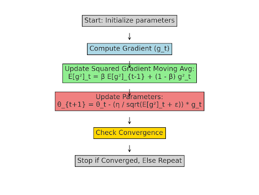
Compute the gradients as partial derivative of the loss function fx with respect to the model parameters at time step t:

fx at xt​ is given by gt=dfdx

Compute the moving average of squared gradients:

E[g²]_t​=βE[g²]_t−1​+(1−β)g²_t

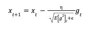
Normalize the Learning Rate:

Where: 

• gt is the gradient of the loss function at time step t.
• E[g^2]t ​ is the exponentially decaying average of past squared gradients.
• β (typically 0.9) controls the decay rate.
• ϵ epsilonϵ is a small constant to prevent division by zero.
• ηis the learning rate.
• The denominator ensures that the update step is scaled down for large gradients and scaled up for small gradients.

More on Machine LearningMean Squared Error (MSE) vs. Mean Squared Logarithmic Error (MSLE): A Guide

RMSProp Steps

1. Compute the Moving Average of Squared Gradients

Instead of using the raw gradient gt​, RMSprop keeps track of the squared gradient using an exponentially decaying moving average: 

E[g²]_t​=βE[g²]_t−1​+(1−β)g²_t

Where:

• gt ​is the gradient of the loss function at time step t.
• E[g^2]t ​ is the exponentially decaying average of past squared gradients.
• β (typically 0.9) controls the decay rate.

2. Normalize the Learning Rate 

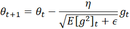
The update rule for RMSprop adjusts the parameter using:

Where:

• ϵ epsilonϵ is a small constant to prevent division by zero.
• ηis the learning rate.
• The denominator ensures that the update step is scaled down for large gradients and scaled up for small gradients.

Why This Works

• Stabilized Updates: Large gradients result in smaller updates, preventing drastic changes in parameters.
• Adaptive Learning Rate: Parameters with consistently large gradients have reduced step sizes, while parameters with small gradients retain a relatively larger learning rate.
• Better Convergence: Helps training on complex landscapes with varying curvature by smoothing updates.

RMSProp Example

Let’s take a simple example to see how RMSprop works in practice. Suppose we are trying to minimize a function fx using RMSprop.

1. Enter Data

• Initial parameter: x0=2.0
• Learning rate: η=0.1
• Decay rate: β=0.9
• Small constant: ϵ=10-8
• Gradient at each step: We assume the gradient of the function fx at xt​ is given by gt=dfdx

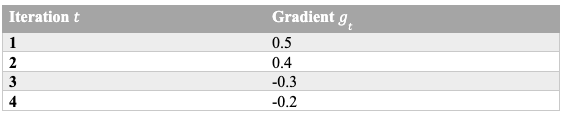
Let’s assume the gradient values at each step:

 

2. Compute RMSprop Updates

RMSprop maintains a moving average of squared gradients:

E[g²]_t​=βE[g²]_t−1​+(1−β)g²_t

The parameter update rule is:

Let’s calculate this for a few steps.

Iteration 1

E[g²]₁ = 0.9(0) + (1 - 0.9)(0.5²) = 0.025

x₁ = 2.0 - (0.1 / √(0.025 + 10⁻⁸)) × 0.5

x₁ = 1.842

Iteration 2

E[g²]₂ = 0.9(0.025) + (1 - 0.9)(0.4²) = 0.0325

x₂ = 1.842 - (0.1 / √(0.0325 + 10⁻⁸)) × 0.4

x₂ = 1.762

Iteration 3

E[g²]₃ = 0.9(0.0325) + (1 - 0.9)(-0.3²) = 0.0344

x₃ = 1.762 - (0.1 / √(0.0344 + 10⁻⁸)) × (-0.3)

x₃ = 1.916

Iteration 4

E[g²]₄ = 0.9(0.0344) + (1 - 0.9)(-0.2²) = 0.0325

x₄ = 1.916 - (0.1 / √(0.0325 + 10⁻⁸)) × (-0.2)

x₄ = 2.027

Advantages of RMSprop

• Adaptive Learning Rates: Unlike standard gradient descent, RMSprop adjusts learning rates dynamically, helping to maintain stable convergence.
• Better Handling of Non-Stationary Problems: Ideal for reinforcement learning and RNNs, where loss landscapes can change over time.
• Faster Convergence: By smoothing gradient updates, RMSprop avoids oscillations and speeds up training.

Limitations of RMSProp

• The choice of the decay factor (β) and learning rate (η) can significantly impact performance.
• It does not consider momentum directly, unlike Adam, which combines RMSprop with momentum.

RMSProp vs. Adam

Both RMSprop and Adam dynamically adjust learning rates for each parameter, but they differ in how they update gradients.

RMSprop

RMSprop uses an exponentially decaying average of squared gradients to normalize updates:

E[g²]_t​=βE[g²]_t−1​+(1−β)g²_t

This stabilizes training by dampening oscillations, making it effective for non-stationary problems like RNNs and reinforcement learning.

Adam

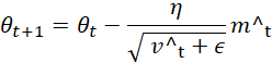
Adam improves on RMSprop by adding momentum, tracking both the moving average of gradients and squared gradients:

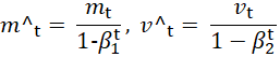
Where:

• is the gradient of the loss function at time step
• ​ is the moving average of the gradient, acting as momentum for smoother updates.
• ​ is the moving average of the squared gradient, normalizing learning rates.
• ​is the decay rate for momentum (commonly 0.9), controlling how past gradients affect updates.
• ​is the decay rate for squared gradients (commonly 0.999), ensuring stability.
• ​,are the bias-corrected versions of ​ and ​, compensating for initial underestimation.
• η is the learning rate, defining step size for parameter updates.
• ϵ is the small constant (e.g., 10^-8) to prevent division by zero.
• ​ is the model parameters (weights) at time step  

Adam balances speed and stability, making it a better general-purpose optimizer than RMSprop.

More on Machine LearningHow Loss Functions Work in Neural Networks and Deep Learning

RMSProp vs. Standard Gradient Descent

Gradient descent updates the parameters of a model by computing the gradient of the loss function with respect to each parameter. The standard update rule in SGD is:

Where:

• θt​ represents the parameter at time step t.
• η is the learning rate (a fixed value).
• gt is the gradient of the loss function at t.

Issues with SGD:

• Sensitive to Learning Rate Choice: A large η can cause the model to overshoot the minimum, while a small η slows convergence.
• Oscillations in Training: If the loss function has steep and shallow directions, the gradient updates can vary significantly, leading to instability.

To address these limitations, advanced optimization techniques introduce adaptive learning rates and momentum-based updates. Among these, RMSprop stands out as a widely used method for stabilizing training and speeding up convergence.

RMSprop improves upon standard SGD by adjusting the learning rate dynamically for each parameter. Instead of using a fixed learning rate, it maintains a moving average of squared gradients to scale updates, preventing drastic fluctuations. This technique is particularly useful for models dealing with sparse or noisy gradients, such as recurrent neural networks (RNNs).

Comparison with Other Optimizers

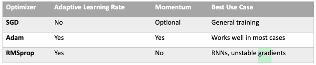
RMSprop is a powerful optimization algorithm that stabilizes training in deep learning models, particularly for problems with high variance in gradients. While Adam is often preferred for general-purpose deep learning tasks, RMSprop remains a strong choice for recurrent networks and reinforcement learning applications.

Frequently Asked Questions