Partial Least Squares Regression (PLS)

Partial least squares regression is a powerful method for analyzing complex relationships among multiple variables, particularly in high-dimensional data sets. You can apply it to a variety of fields, such as business, science, bioinformatics and anthropology.

PLS regression is particularly useful when predictor variables are highly correlated with each other or when the number of predictors exceeds the number of observations (cases where regression assumptions violations cause OLS to provide unstable results).

More by This AuthorHow to Evaluate Large Language Models

What Is PLS Used For?

PLS regression finds the latent factors underlying the independent variables that explain variance in some dependent variables. For example, marketers use it to model consumer behavior and assess factors influencing customer satisfaction and loyalty. In finance, PLS aids in predictive analytics, allowing for better risk management and decision-making processes.

The methodology’s flexibility in dealing with different types of data and its capacity for simultaneous modeling of multiple dependent variables contribute to an increasing prominence in business analytics.

Additionally, PLS can produce robust predictions even with small sample sizes; you can enhance this with cross-validation, determining the optimal number of components and minimizing the risk of overfitting.

Components of Partial Least Squares

PLS regression works by constructing new predictor variables (components) as linear combinations of the original predictor variables. We extract components to explain as much of the covariance between the predictor variables and the response variable as possible.

Selecting an appropriate number of components is essential to prevent overfitting and ensure the model’s generalizability.

There are two key sets of variables:

• Exogenous (predictor) variables are the independent variables used to explain or predict an outcome.
• Endogenous (response) variables are the dependent variables of interest.

PLS creates latent variables (components) for the predictor variables, capturing the most relevant information to explain the variability in both sets, paving the way for robust and predictive modeling.

How Does PLS Work?

PLS regression is a three-step process.

1. Dimensionality Reduction

We extract components that maximize the explanation of the covariance between the predictor variables and the response variable. We select these components to explain as much of the covariance between the predictor variables and the response variable as possible.

2. Regression

Researchers regress the response variable on the latent variables. PLS uses least-squares regression on these components to predict the response variables.

3. Cross-Validation 

Cross-validation determines the optimal number of components, ensures the model’s generalizability, and prevents over-fitting.

The PLS algorithm starts by extracting the direction in the space of the Xs that explains the maximum variance in the Ys; this is the first component. The NIPALS (nonlinear iterative partial least squares) algorithm sequentially adds components, each explaining the maximum variance in the Ys orthogonal to the previous components.

Partial Least Squares Regression Example

Consider a marketer who wants to understand customer lifetime value. They consider many factors, but traditionally, they use a combination of RFMV (recency, frequency, monetary value, variety) and demographics.

These features are multicollinear, so traditional ordinary least squares may fail.

I have built a typical marketing data set representing 500 customers.

# Separate features (X) and target (y)
df_scale = StandardScaler().fit_transform(df)
df_scale = pd.DataFrame(df_scale, columns=df.columns, index=df.index)

X_scaled = df_scale.drop('CLTV', axis=1)
y_scaled = df_scale['CLTV']

# Split data into training and testing sets
X_train_scaled, X_test_scaled, y_train_scaled, y_test_scaled = train_test_split(X_scaled, y_scaled, test_size=0.2, random_state=1)

# Create the cltv_train dataset
cltv_train = X_scaled[['Recency', 'Frequency', 'MonetaryValue']].copy()
cltv_train['CLTV'] = y_scaled.copy()
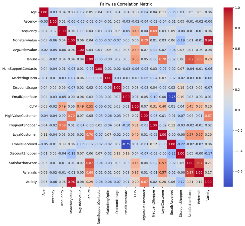
other_train = X_scaled.drop(['Recency', 'Frequency', 'MonetaryValue'], axis=1)

The pairwise correlation heatmap shows that our features correlate well with CLTV and each other.

Using k-fold cross-validation, I iteratively extract different numbers of components, create the regression model and measure the mean-squared error. A plot of the MSE versus the number of components informs my selection of the fewest components that provide a low error.

# --- Variable Importance in Projection ---

def VIP(pls_model):
    """
    Calculates VIP scores for a PLS model.
    Args:
        pls_model: Fitted PLSRegression object.
    Returns:
        Array of VIP scores for each feature.
    """
    t = pls_model.x_scores_
    w = pls_model.x_weights_
    q = pls_model.y_loadings_
    p, h = w.shape  

    # Calculate VIP scores for each feature
    vips = np.zeros(p)
    s = np.diag(np.dot(t.T, t))  
    for i in range(p):
        for j in range(h):
            vips[i] += (w[i, j]**2 * s[j]) * (q[0,j]**2 / np.sum(q**2 * s))
    vips = np.sqrt(p * vips)
    return vips

# --- Find optimal number of PLS components ---

# Define the range of components to test
n_components_range = range(1, X_train_scaled.shape[1] + 1)

cv_mse = []

# Perform cross-validation for each number of components
for n_components in n_components_range:
    pls = PLSRegression(n_components=n_components)
    kf = KFold(n_splits=5, shuffle=True, random_state=1)
    mse_scores = []
    for train_index, val_index in kf.split(X_train_scaled):
        X_train_cv, X_val_cv = X_train_scaled.iloc[train_index], X_train_scaled.iloc[val_index]
        y_train_cv, y_val_cv = y_train_scaled.iloc[train_index], y_train_scaled.iloc[val_index]
        pls.fit(X_train_cv, y_train_cv)
        y_pred_cv = pls.predict(X_val_cv)
        mse_scores.append(mean_squared_error(y_val_cv, y_pred_cv))
    cv_mse.append(np.mean(mse_scores))

# Find the optimal number of components with the lowest MSE
optimal_n_components = n_components_range[np.argmin(cv_mse)]
print(f"Optimal number of PLS components: {optimal_n_components}")

# --- PLS Regression ---
pls = PLSRegression(n_components=optimal_n_components)  
pls.fit(X_train_scaled, y_train_scaled)
y_pred_pls = pls.predict(X_test_scaled)
mse_pls = mean_squared_error(y_test_scaled, y_pred_pls)
r2_pls = r2_score(y_test_scaled, y_pred_pls)

print("PLS Regression:")
print(f"  Mean Squared Error: {mse_pls:,.2f}")
print(f"  R-squared: {r2_pls:.2f}")

# --- Diagnostics and Component Explanation ---
# 1. Explained variance in X and Y
explained_variance_X = np.var(pls.x_scores_, axis=0) / np.var(X_train_scaled, axis=0).sum()
explained_variance_Y = np.var(pls.y_scores_, axis=0) / np.var(y_train_scaled, axis=0)

print("\nExplained Variance in X (by component):", explained_variance_X)
print("Explained Variance in Y (by component):", explained_variance_Y)

# 2. VIP scores (Variable Importance in Projection)
vip_scores = VIP(pls)

# 3. PLS component loading
component_df = pd.DataFrame(component_weights, index=X_train_scaled.columns, columns=[f"Component {i+1}" for i in range(pls.n_components)])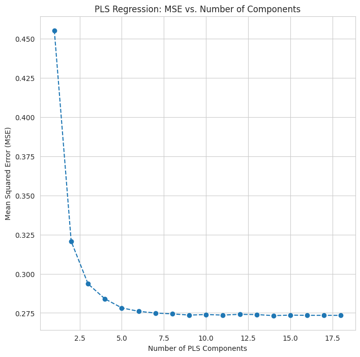

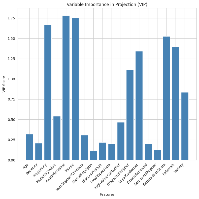
In this data set, I select six components, yielding a model with an MSE of 0.26 and an R-squared of 0.71. Because the components are linear combinations, interpretation is more complex than OLS. Variable importance in projection tells us which features have the highest loadings across all the components.

Here’s another helpful visualization is a heatmap of loadings by component.

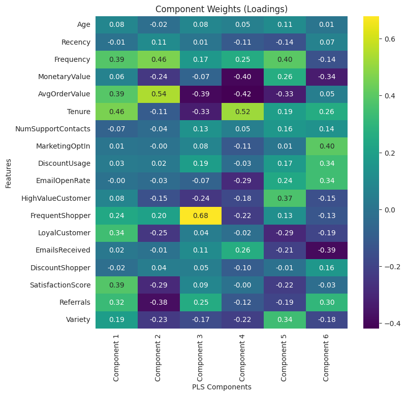
With these loadings, we can describe the latent variables. For example, component three represents frequent shoppers with short tenure and low order sizes.

More on RegressionWhat Is Logistic Regression?

Partial Least Squares Versus Other Models

PLS regression shares characteristics with other regression and feature transformation techniques. Here’s how it compares to some other standard methods.

Multivariate Multiple Regression

Multivariate multiple regression models multiple responses, or dependent variables, with a single set of predictor variables. Unlike multivariate multiple regression, which focuses on modeling multiple response variables, PLS regression focuses on finding a relationship between two sets of variables by reducing the dimensionality of the predictor variables. PLS is more flexible in handling complex data structures such as collinearity. With only one dependent variable, MMR becomes OLS.

Principal Components Regression

Principal component regression is a technique that uses principal component analysis to reduce the dimensionality of the data before performing regression. While both PLS and PCR aim to reduce the dimensionality of the data, they differ in how they select the components.

PCR selects components that capture the most variance in the predictor variables, while PLS selects components that capture the most covariance between the predictor and response variables. This key difference makes PLS more suitable for predictive modeling, as it focuses on relevant components to the response variable.

# --- Principal Component Regression (PCR) ---
pca = PCA(n_components=optimal_n_components)  # Using the same number of components as PLS for comparison
X_train_pca = pca.fit_transform(X_train_scaled)
X_test_pca = pca.transform(X_test_scaled)

pcr = LinearRegression()
pcr.fit(X_train_pca, y_train_scaled)
y_pred_pcr = pcr.predict(X_test_pca)
mse_pcr = mean_squared_error(y_test_scaled, y_pred_pcr)
r2_pcr = r2_score(y_test_scaled, y_pred_pcr)

# 1. Explained Variance Ratio:
explained_variance_ratio = pca.explained_variance_ratio_

# 2. PCA loadings
loadings = pca.components_
num_features = X_train_scaled.shape[1]
feature_names = X_train_scaled.columns
pc_loadings = pd.DataFrame(loadings.T, index=feature_names, columns=[f"PC{i+1}" for i in range(pca.n_components)])

First, let’s look at a scree plot of the number of principal components and the amount of variance explained.

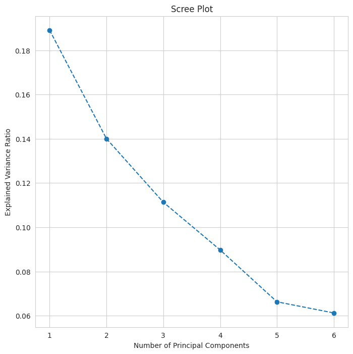
Six components should suffice, and a six component PCR produces a model with an MSE of 0.53 and an R-squared of 0.41. Principal components are not selected with the dependent variable in mind, so, unsurprisingly, the PCR model does not explain as much variance as PLS. A key difference is that PLS is a supervised method, accounting for the response variable when transforming, while PCA is largely unsupervised, focusing solely on maximizing variance. 

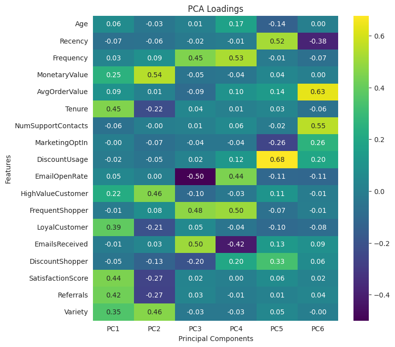
Interpretability is similar to PCS: we look at the component loading and try to make sense of it. Component one is long-tenured, highly satisfied customers that make referrals.

Canonical Correlation Analysis

Canonical correlation analysis is another statistical method for finding linear relationships between two sets of variables. Both techniques create latent variables.

CCA focuses on maximizing the correlation between the two variables, while PLS focuses on maximizing the covariance. You can view PLS as a generalization of CCA, which is more suitable for predictive modeling because it considers the magnitude of the relationships between the variables.

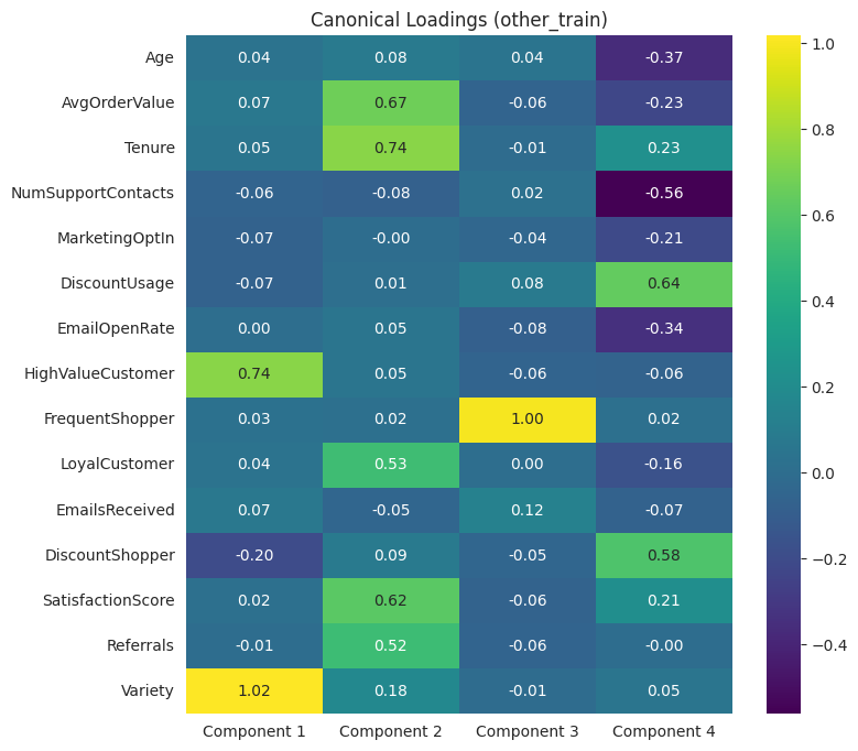
For the example data, I separated the features into two groups: a CLTV group with CLTV, recency, frequency and monetary value, and an Other group with all remaining variables.

CCA can produce as many canonical variables as there are features in the smaller group, which, in this case, is four.

# --- Canonical Correlation Analysis (CCA) ---

# Initialize CanCorr object
cca = CCA(scale=False, n_components=4)  
cca.fit(cltv_train, other_train)
cltv_c, other_c = cca.transform(cltv_train, other_train)

# Calculate and visualize correlations
comp_corr = [np.corrcoef(cltv_c[:, i], other_c[:, i])[1][0] for i in range(cca.n_components)]

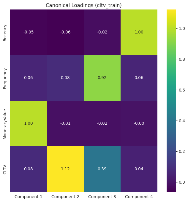
# 1. CCA loadings (weights)
cltv_loadings = pd.DataFrame(cca.x_loadings_, index=cltv_train.columns, columns=[f"Component {i+1}" for i in range(cca.n_components)])
other_loadings = pd.DataFrame(cca.y_loadings_, index=other_train.columns, columns=[f"Component {i+1}" for i in range(cca.n_components)])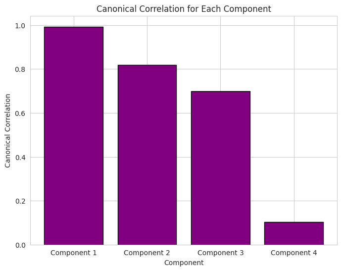

Now, we can look at the loadings in each group.

Applications of PLS

Researchers in various domains favor PLS for identifying strong predictors in large sets of correlated variables. The choice of strong predictors can help focus organizational efforts in business, leading to more data-driven decision-making. Many firms successfully apply PLS regression in areas such as marketing, finance and sales.

Marketing

Evaluate the impact of promotional efforts on customer satisfaction and loyalty while controlling for numerous demographic and psychographic variables.

Finance

Predict market volatility using macroeconomic indicators and financial ratios that frequently correlate highly.  

Sales 

Forecast revenue by combining internal sales data, marketing inputs and external competitive factors such as competitor pricing strategies

When to Use Partial Least Squares Instead of Ordinary Least Squares

OLS regression is the most common statistical method for estimating the parameters of a linear regression model. It’s problematic, however, when there’s multicollinearity among the predictor variables or when the number of predictors exceeds the number of observations.

In these cases, PLS regression offers a more robust alternative. Using all PLS components provides an equivalent fitting model to OLS. 

In the example data set we don't have perfect multicollinearity, which would prevent OLS from running, so I fit an OLS model. The model has an MSE of 0.27 and an R-squared of 0.70. However, the regression diagnostics tells us that many of the features are not significant in the model.

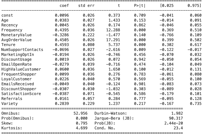
Checking the linear regression assumptions reveals many violations.

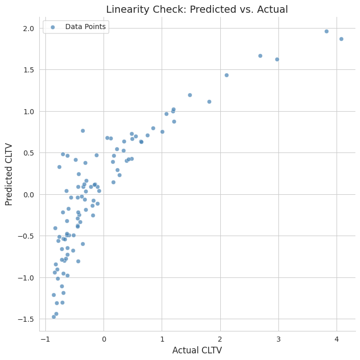
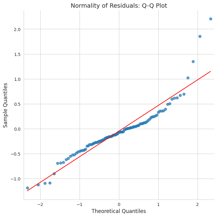
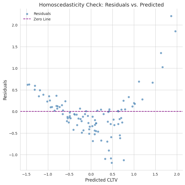
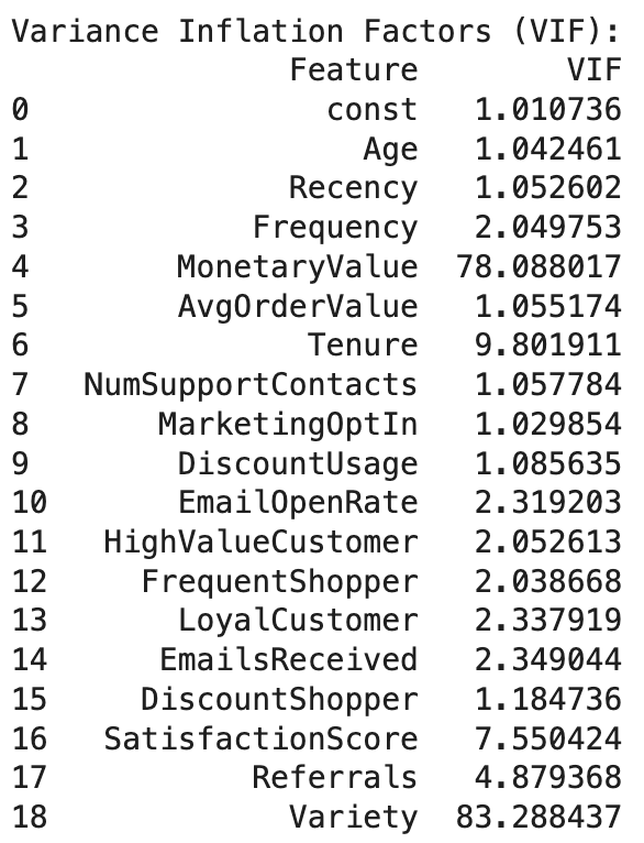
The assumption violations and non-significant parameter estimates let us know that OLS is inappropriate unless we drop some features and potentially transform others.

Frequently Asked Questions