What Is Overfitting?

In machine learning, overfitting is a problem that results from attempting to capture every variance in a data set. An overfit model will lead to major errors when deployed to production, causing inaccurate predictions and unreliable results. In this article, we’ll explore what causes overfitting in the machine learning model development process and how to fix it to ensure your machine learning projects are reliable.

More in Machine LearningUnsupervised Clustering: A Guide

 

Bias and Variance in Machine Learning

Before we dive into overfitting, it’s important to understand the roles bias and variance play in designing accurate machine learning models.   

Bias

Bias is an error that occurs when a machine learning model makes assumptions about the training data to simplify the learning process, failing to gather enough information from the data. High bias can lead to the model performing poorly with both training data and testing data, which is known as underfitting.

Thinking about bias in mathematical terms, let’s define the model error (e) as the difference between the actual value and the predicted value: e = (y – ŷ). Here, y is the actual value and ŷ is the predicted value. The bias is the difference between the actual value (y) and the expected value from the model. In other words: Bias measures the systematic error when the model consistently misses the target. 

Figure five demonstrates the meaning of the bias using a target practice analogy, where the target’s inner circle represents low bias:

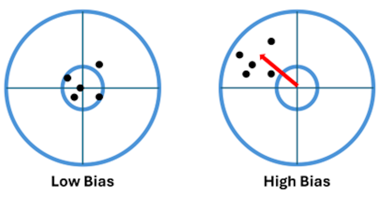
In the case of high bias in the target on the right, the relative distribution of the model predictions did not change, but their overall location shifted because of the bias. 

Variance

Variance is an error that occurs when a machine learning model is overly sensitive to its training data, picking up noise along with patterns in the training data. The model will perform well on the training data, but won’t perform well with testing data when the variance is high — what’s known as overfitting. 

In mathematical terms, variance is the average of the square of the deviation of the predicted value from the mean predicted value. In other words: It is the variance (square value of the standard deviation) of the predicted values. It measures the amount of scatter of the predicted values around a central expected value. Figure six shows the target practice analogy in the case of low and high variance: 

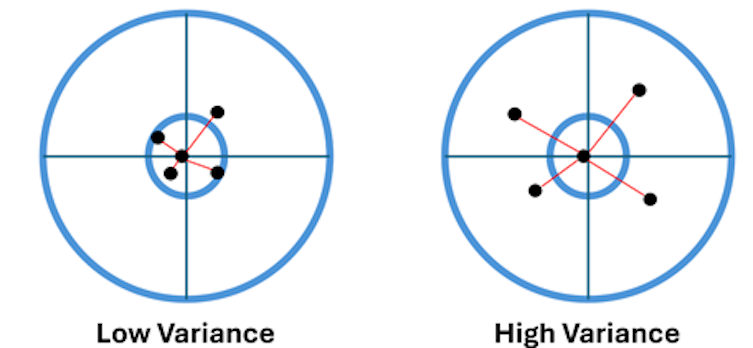
Figure six shows that the location of the center of the model predictions did not change, but the scatter around this center increased in the case of higher variance. 

An example of how to measure the model prediction error is the mean square error (MSE) of the model, which is the average value of the squared difference between the actual and predicted value. The MSE can be deconstructed into the three components as follows: MSE = Bias(ŷ)² + Variance(ŷ) + Irreducible Error. Here, irreducible error represents the limit of the variables in the model to predict the target value. 

Predicted values and actual values are at the heart of loss curves, which calculate the difference between a model’s predicted value and the actual value to see how far away a model is from the correct value. A loss curve consists of every output for the training and testing data, so we can compare how the model performs with each. In an ideal situation, the graph for the training data will slope down and plateau while the graph for the testing data will behave similarly before sloping back up, signaling improved performance over time. 

When we minimize bias and variance, we end up with a well-fit model. Model fitting is the process of determining how well a machine learning model performs on data similar to its training data. This ability to generalize across different data sets hinges on reducing bias and variance as much as possible. Generalization is ultimately what we’re striving to achieve when training machine learning models. Once we have a well-fitted model, we can use it to analyze different data and make accurate predictions.

Applications of Machine Learning8 Advancements Changing the World of Search

 

What Is Overfitting? 

Overfitting refers to a machine learning model that makes accurate predictions when using its training data, but performs poorly when using new data sets. There are a number of factors that can lead to overfitting, with the most common being: 

• Data sets filled with too much noise that the model mistakes for actual patterns.
• Small data sets that don’t contain a wide enough variety of data. 
• Training a model on a single data set for too long. 
• Models that are overly complex and learn too many parameters from the training data.   

In all these cases, a machine learning model may learn the details of a data set to the point that it becomes a near-exact fit of the data. This means it has merely memorized particular data points instead of learning general patterns. As a result, it cannot generalize what it has learned and apply these lessons to other data sets, limiting its accuracy to the training data set. 

The lack of generalization that results from overfitting can have lasting consequences in real-world scenarios. Consider a model trained to analyze medical images and determine whether a disease is prevalent or not. An overfit model may incorrectly diagnose patients with a disease and incorrectly say patients are healthy when they actually do have the disease. Or take a model that’s trained to predict stock prices. In this case, an overfit model could deliver inaccurate predictions that lead to bad investments and financial losses.    

Although many machine learning model development methodologies exist, they all include the steps shown below: 

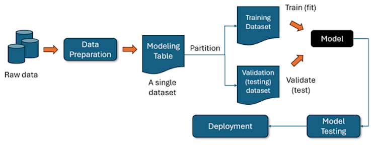
This image represents the typical workflow of building and deploying a machine learning model. Let’s break it down step by step:

1. The process starts with raw data gathered from databases, sensors or other inputs. 
2. The data is then cleaned, transformed and formatted to make it understandable for machine learning models. 
3. The processed data is stored in a structured format, often referred to as a modeling table. This dataset contains features and target variables for training and validation.
4. The dataset is then split into training data — used to train (fit) the model, helping it learn patterns and relationships — and testing data — used to test (validate) the model’s performance by evaluating how well it performs with new data.
5. The model is trained using the training dataset, learning to minimize error and maximize accuracy based on the chosen algorithm.
6. The model is then tested using the validation dataset to assess its performance. This helps in fine-tuning hyperparameters and preventing overfitting. Methods like grid search, random search and Bayesian optimization are used for tuning hyperparameters.
7. Once the model is accurate, it is deployed into a real-world environment where it can make predictions on new data.
8. Even after deployment, the model undergoes continuous testing to ensure it remains accurate and reliable.

In the model fitting (or training) step, we use the training data set to fit the model and the validation data set to assess its quality. At this phase of the process, the problem of overfitting can occur. Model overfitting — or underfitting — affects the quality of a model. A good machine learning model must be: 

1. Accurate
2. Robust
3. Small (parsimonious)
4. Explainable

Achieving these four attributes in any model is not straightforward, however. Improving the accuracy of the model fitted using the training data set usually comes at the expense of the other three characteristics, as shown in figure two: 

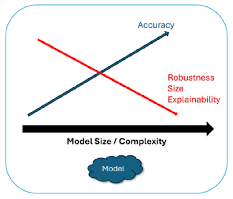
The image above illustrates this trade-off. As machine learning models increase in size and complexity, they become more accurate because they can capture more detailed relationships within the data. At the same time, larger and more complex models are harder to maintain because they’re so resource-intensive. Plus, it’s difficult to understand how they reach their conclusions. This makes them less robust than smaller models, which are simpler but excel at generalization. 

Improving accuracy while fitting the model on the training data set could then result in overfitting, which leads to high prediction errors when we test the model using the validation data set. It also increases the size and complexity of the model, reducing our ability to explain the meaning behind data analytics predictions. 

Overfitting Real-Life Example

Let’s explain this through a simple example. A shipping company that ships parcels would like to develop a model to calculate the cost of shipping parcels (y) in terms of: 

• The shipping distance in miles (x)
• The weight of the parcel in pounds (w)
• The volume of the parcel in square feet (h) 

An example of a small, simple model would be y = 15 + 5x. An example of a slightly more complex model with more variables would be y = 15 + 5x + yh + 8w. Finally, an example of a complex model with the same three variables would be:

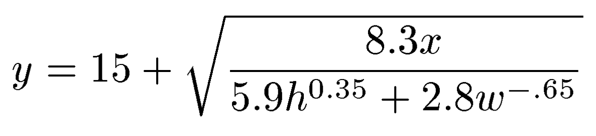
Note that these are not actual models, merely examples.

Overfitting Code-Based Example

Let’s take a look at another example, this time using Python code in scikit-learn. To get started, we create some synthetic data based on a cubic equation with added noise to simulate real-world randomness.

import numpy as np
import matplotlib.pyplot as plt
from sklearn.model_selection import train_test_split
from sklearn.preprocessing import PolynomialFeatures
from sklearn.linear_model import LinearRegression
from sklearn.metrics import mean_squared_error

# Step 1: Generate synthetic data
np.random.seed(42)
X = np.linspace(-3, 3, 100).reshape(-1, 1)
y = X**3 - 3*X**2 + 2*X + np.random.normal(0, 2, size=X.shape)  # Cubic function + noise

Next, we split the dataset into training (80 percent) and testing (20 percent), so we can see how well the model generalizes.

# Step 2: Split data into training and testing sets
X_train, X_test, y_train, y_test = train_test_split(X, y, test_size=0.2, random_state=42)

# Function to fit models with different complexities
def evaluate_model(degree):

We then apply polynomial transformations to capture non-linearity (higher degrees allow more complex patterns).

    # Step 3: Transform features into polynomial features
    poly = PolynomialFeatures(degree=degree)
    X_train_poly = poly.fit_transform(X_train)
    X_test_poly = poly.transform(X_test)

We fit a simple linear regression model to the transformed features.

    # Step 4: Train a linear regression model
    model = LinearRegression()
    model.fit(X_train_poly, y_train)

The trained model makes predictions for both the training and test datasets.

    # Step 5: Make predictions
    y_train_pred = model.predict(X_train_poly)
    y_test_pred = model.predict(X_test_poly)

We can then calculate the mean squared error for both training and testing datasets.

    # Step 6: Compute errors
    train_error = mean_squared_error(y_train, y_train_pred)
    test_error = mean_squared_error(y_test, y_test_pred)

    print(f"Degree: {degree} | Train Error: {train_error:.2f} | Test Error: {test_error:.2f}")

We repeat the process for different polynomial degrees, as depicted in the graphs below:

# Step 7: Evaluate models with different degrees
for degree in [1, 3, 10]:  # Trying low (underfit), optimal, and high (overfit) degrees
    evaluate_model(degree)

For Degree 1, the model is too simple (straight line) and cannot capture the complexity of the data. It produces a lot of errors during training and testing, so this is a case of underfitting. For Degree 3, the model closely matches the true data distribution, demonstrating low training and test errors. That means it’s a good fit overall and generalizes well. For Degree 10, the model is too complex, capturing noise instead of patterns. It may perform well during training, but it produces many errors when testing with new data. This is a case of overfitting. 

 

Overfitting vs. Underfitting 

In contrast to overfitting, underfitting is when a machine learning model makes inaccurate predictions using both training data and new data sets. This can happen for several reasons: 

• Poorly executed feature engineering — the process of selecting and converting raw data into a readable format for machine learning models. 
• Small training data sets that don’t provide enough parameters. 
• Too much regularization — the process of compensating for overfitting by reducing a model’s accuracy on training data to improve its ability to generalize with new data. 

In each case, the model is oversimplified and unable to identify general patterns in the training data. This leads to poor performance with every data set.  

Let’s now examine in detail what the terms “overfitting” and “underfitting” look like in action. Figure three shows an example of three models fitted to data representing the cost of shipping a parcel (y) versus the shipping distance (x): 

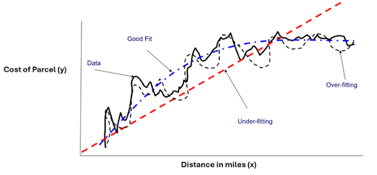
The solid black line is the training data used to fit the models. The red dashed line is a simple model (a straight line in this case), which is clearly an underfit model that would result in large model errors, even on the training data set. 

The black dashed line represents the predictions of a complex model that attempts to capture all the variabilities in the data. This is an overfit model because it would result in large errors when tested using the validation data set. Representing the other extreme of the underfit red dashed line, the overfit model is trying to be too precise. Thus, it misses the data’s broader trends. 

The blue dashed line is considered a good model because it captures the trends in the data without oversimplification and without trying to replicate the data’s every ripple and variation. 

Master Machine LearningUnderstanding the Derivative of the Sigmoid Function

 

How to Detect Overfitting

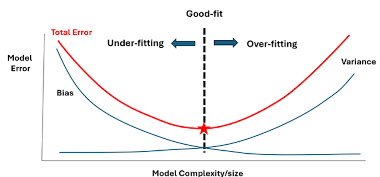
In figure three, we visually assessed the three models and guessed which one could be the best fit to avoid overfitting or underfitting. Another way to visualize these features is shown in figure four: 

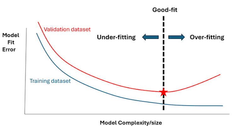
 Figure four shows that increasing the model’s complexity and size by introducing more predictors will result in fewer errors when tested against the training data set — up to a point. After that point, the fit error begins to grow again because the model is beginning to overfit. This threshold represents our dashed blue line in figure three and separates overfitting from underfitting. It is the most appropriate blend of model size and complexity. 

A common method used to detect overfitting is known as k-fold cross-validation, which involves dividing data into ‘k’ equally sized subsets. Once the subsets have been formed, the process goes as follows: 

1. Set aside one subset as the test set, and train the model on the remaining subsets. 
2. Determine how the model performs on the test set.
3. Assign the model a score based on its performance. 
4. Repeat the process until each subset has served as the test set.
5. Calculate the average of the scores to measure a model’s overall performance. 

By cycling through a number of training iterations, k-fold cross-validation makes it less likely that overfitting will occur. You can perform this method using tools like PyTorch, scikit-learn and TensorFlow, although you may need to install some additional libraries. 

 

How to Avoid Overfitting and Underfitting

Avoiding overfitting and underfitting is an important aspect of model development, so most modeling algorithms have developed mechanisms to guard against this problem. The general scheme of all the developed methods follows the strategy shown in figures four and seven. These methods vary the model size and complexity and attempt to minimize the total model error. Most of them are implemented in open-source and proprietary machine learning platforms.

Regularization

Regularization addresses overfitting in machine learning models by cutting down on the number of features. L1 and L2 regularization are two common types, but both go about this process in different ways: 

• L1 regularization: Also known as lasso regression, this type of regularization penalizes weights to the point of bringing some down to the value of zero. This removes features deemed unnecessary from the model.  
• L2 regularization: Also known as ridge regression, this type of regularization penalizes weights by the squared magnitude of the coefficient. This makes all weights smaller, but it doesn’t fully remove any features. 

In the case of any regularization method, the goal is to either reduce unnecessary noise in the data or prevent the machine learning model from becoming too complex. Keeping the model simple supports generalization.  

Ensemble Learning

Ensemble learning is an approach that combines the results of several weaker machine learning models to create a stronger model that delivers more accurate results. When it comes to ensemble models, there are two main types to know: 

• Bagging: Produces multiple training sets by selecting and replacing data points — meaning data points can be selected more than once. Models are then trained separately on different versions of the training data, and the average of these models’ predictions is calculated to find a more accurate prediction. 
• Boosting: Instead of training multiple models at once, boosting trains one model at a time. Also unlike bagging, boosting selects the data points misclassified in the previous iteration for the next iteration. The process is repeated, and the results of each iteration are combined to generate a more accurate prediction. 

Employing several machine learning models inherently leads to more generalized results, as opposed to just one model. And using different versions of data sets makes it harder for models to become too fitted to a particular data set, avoiding overfitting.    

Decision Trees

Decision trees use a tree-like structure to represent a series of tests and outputs, with the final prediction being the sum of all these outputs. This process is designed to find the optimal value. However, decision trees tend to overfit when they become large. Terminal nodes end up with a small number of records, so predictions based on these small samples are not robust. Therefore, many pruning algorithms have been developed to minimize the total error, as previously shown in figure seven. 

Pruning algorithms remove unnecessary parts of a decision tree. By eliminating excessive data, pruning can reduce noise in the data and improve a model’s training process. You can perform tree pruning while generating the splits by eliminating those splits that increase the total error on a validation data set. Alternatively, a pruning algorithm would grow a large tree and then prune it back to reduce the error. 

More recently, advanced decision tree algorithms have been equipped with features to handle overfitting and pruning tasks. Here are just a few algorithms to know: 

XGBoost

Short for eXtreme Gradient Boosting, XGBoost uses the technique of gradient boosting — combining several weak models to create a strong model that delivers more accurate predictions. XGBoost comes with a number of adjustable parameters to prevent overfitting. For example, users can set the maximum depth of a decision tree and lower the ratio of the training instances involved to reduce the chances of overfitting. 

LightGBM

Short for Light Gradient-Boosting Machine, LightGBM is known for its speed and supports graphics processing unit (GPU) learning to further increase its computational power. It also has adjustable parameters, most notably the minimum number of data points that a leaf node in a decision tree must have before splitting and the maximum tree depth. 

CatBoost 

CatBoost is an open-source library that minimizes the amount of preprocessing required when addressing categorical data. The tool comes with its own overfitting detector that can be tailored to classification and regression problems. 

Regression Models

Regression models seek to establish relationships between variables. These models and their derivatives have been around for a long time, with several schemes having been introduced to find the optimal model. These schemes depend on inserting and removing the predictors in a specific order to hunt for the minimum error. 

For example, in the forward variable selection method, the predictors are inserted one at a time so that the variable with the expected highest increase in model accuracy is used in each step. The process stops when no predictor can significantly improve the model’s accuracy. 

The backward scheme is just the opposite of the forward scheme. We start with a model with all the possible predictors and then remove them one by one. A hybrid scheme known as the stepwise selection method works by inserting and removing variables iteratively until the best model is attained. Other model development schemes rely on using a measure of model accuracy, such as the R² to add and remove variables iteratively in each step. 

Neural Networks

Neural networks, in specific multilayered perceptron networks, are trained by iteratively adjusting the values of the weights between the neurons in the different layers. During the training iterations, commonly known as epochs, the weights change and the network minimizes the errors on the training data set with each epoch. The prediction error on the validation data set will be as in figure four. Sometimes the validation data error may not be unimodal, however. This means that it may have more than one minimum. This is shown in figure eight:  

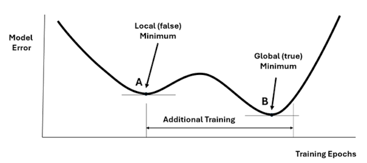
To ensure that the model fitting process captures the global minimum and not just a local one, after finding a minimum (point A), the training is resumed for a number of epochs to ensure that we actually found the global minimum (point B). Although this simple strategy does not guarantee finding the global minimum’s location, it is usually sufficient for most practical cases. 

There are several other techniques that neural networks can use to help reduce overfitting: 

• Learning rate schedules: Adjust the learning rate of a model between each iteration, usually using a higher learning rate early to prioritize learning general patterns before decreasing the rate later on to prioritize accuracy. This process reduces the chances of a model absorbing noise.  
• Adam optimization algorithm: Customizes the learning rates of each parameter and comes with bias correction terms. This algorithm helps a neural network train efficiently and ignore noise in the data.  
• Dropout: Involves randomly selecting neurons to temporarily drop out for an iteration during training. This forces a neural network to use all neurons when learning, so it doesn’t rely too much on specific neurons and become overfit as a result. 
• Weight decay: Penalizes larger weights in a neural network, encouraging the network to use smaller weights. This prevents the model from becoming too complex and encourages it to learn from many connections, leading to generalized learning.
• Early stopping: Stops a neural network’s training when the network has reached peak performance with a specific data set and its performance has started to worsen. This ensures it learns generalizable patterns without picking up noise from the data. 

Data Augmentation

Data augmentation refers to tweaking the sample data during each iteration of a machine learning model’s training. This leads the model to treat each version of the sample data as new or unfamiliar data. It then doesn’t learn too closely the exact details of a data set, instead learning general patterns it can apply to different data sets. 

Feature Selection

Feature selection is the process of determining which features in the training data are the most important and then removing features that are repetitive or unimportant. This cuts down on the noise within a data set. Although this is similar to pruning, these two techniques are not the same. Feature selection focuses on the most important features while pruning emphasizes the most irrelevant features. 

Frequently Asked Questions